 Expected Monitory Value (EMV) analysis is part of risk analysis process. This is used to calculate cost of each decision alternatives available in the project to choose the cost effective and best decision, using Decision Tree analysis.
This is typically used during the exercise to prioritize risks based on quantitative risk analysis.
This statistical analysis tool is about coming up with possible scenarios to deal with a risk and assessing how much each of those paths will cost the project against the benefits, and letting you choose the best possible path which has lesser risk and higher benefit.
Expected Monitory Value of a project = Sum of (every possible outcome x probability of the outcome happening)
If this looks cryptic, do not worry. This is done easily with visual aid, called Decision Tree.
What is a decision tree?
A decision tree is a decision support tool to decide on a strategy that is most likely to reach the costs-versus-benefits goal.
Refer to the figure below. Decision tree is a tree like graph of decisions and their possible consequences. At each decision point you multiply probability of that decision occurring, with cost associated with that decision, and get a value.
When you are done plotting this graph you will have several paths (or branches) through the decision tree reaching conclusions. Now you sum up the numbers (payoffs minus costs) along each of these paths and the number you get for each path is the net path value.
From this then you will be able to calculate EMV value at each decision node. The best decision path to go with usually is the one with highest number for net path value among all the decision branches.
A simpler analogy to understand Decision tree could be this –
Let us say you want to find the best route from home to your new office. The shortest route may not necessarily be the one with least cost or best route.
As you drive from home, at each junction you will have multiple roads that can be taken. Going by each road will have its own cost (gas, time, traffic, road condition, driving stress, wear & tear of car) and a certain probability of reaching office on time.
This way you will plot several possible routes to reach office – and each route will have an associated total cost. You could then decide on the best route – that costs you least, benefits most and makes for a comfortable ride.
Decision tree has three types of nodes:
- Decision node – represents a decision. Shown with a rectangle. Decision is written inside this rectangle.
- Chance node – represents uncertainty associated with this decision. Could lead to a payoff or cost. Shown with a circle.
- End node – end of path. Shown with a triangle.
Note that a decision tree has only burst nodes (node from which paths split), and no sink nodes (on which paths converge).
Also read: Sunober shares her study tips and short notes in here.
How do you calculate Expected Monitory Value for a project?
Step 1: Plot the decision tree, you will have more than one possible decision nodes (else you won’t need this tool! 🙂 )
Step 2: For each decision node plot a chance node, with multiple solution possibilities. For each possibility put a probability %value and monitory value representing the benefit. Note that a chance scenario is applicable to all decision nodes.
Step 3: Repeat the steps till you cover all of the possible decisions and their chances, so all of them reach a conclusion end node.
Step 4: For each path, deduct costs from payoffs and write at the end node. You may end up getting a negative value if costs are higher than payoffs.
Step 5: Now to calculate EMV at each decision node working backwards from each end node. Calculate probability of a chance multiplied by net path value of that chance, sum them up for all chances of this decision node. Write this value under the decision node.
Step 6: Now the decision EMV is the largest number among these chance node EMVs calculated at step 5.
If this is not clear, no worries. Let us look at an example.
Kathy’s Landscaping project has an all-season theme park for which she needs exotic plants in large quantities. She has two choices – either buy from a plant nursery or grow internally at their facilities.
Let us see how she can come to a decision based on Expected Monitory Value of each decision, using a decision tree: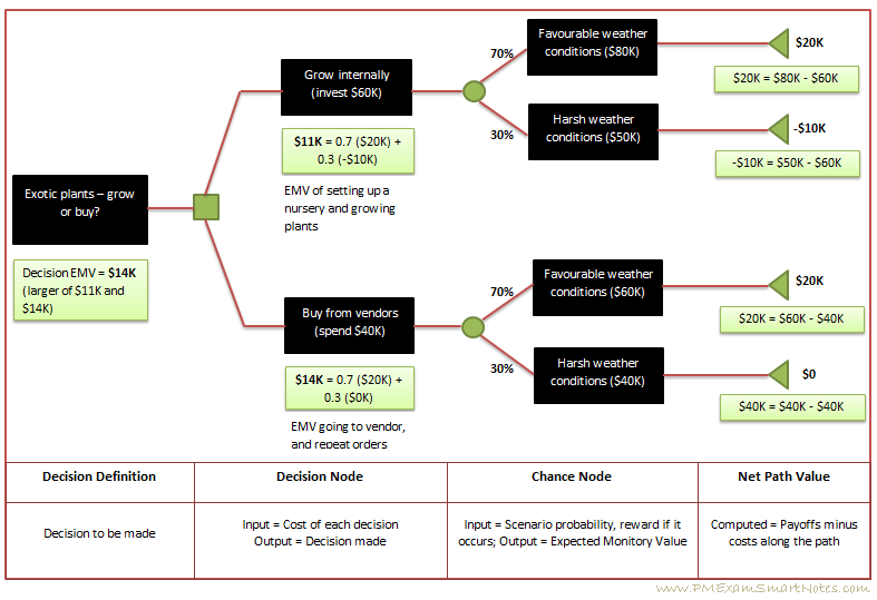
Figure: Expected Monitory Value calculation using Decision Tree tool
The volume of exotic plants needed for the theme park is large. Hence Kathy had to decide whether to set up an internal nursery and grow them or buy from outside. Since these are exotic plants some of them might not grow in the weather condition and might need special treatment.
- Growing internally would cost $60K, considering one time set up cost. Buying from outside would cost about $40K.
- For each decision the weather condition (which is uncertain, and therefore represents a ‘chance node’) is to be considered. If weather conditions are favorable Kathy would make a profit of $80K by growing her own plants, while buying from outside she makes only $60K.
- End path value when growing her own plants and weather conditions are favorable, is $20K ($80K – $60K). This is the sum of payoffs minus costs along the path. Similarly Kathy calculates end path values for other branches.
- Expected Monitory Value is calculated at each decision node, multiplying probability of occurrence with end path value for each chance and summing it up. For ‘Grow internally’ decision this turns out to be 0.7 ($20K) + 0.3 (-$10K) = $11K. Similarly the ‘Buy from vendors’ decision this is 0.7 ($20K) + 0.3 ($0K) = $14K.
- Looking at the EMVs, the decision to set up a nursery and grow plants seems to yield lesser Expected Monitory Value, and hence Kathy decides to buy from the vendor (this decision has larger value of EMV, $14K).
Expected Monitory Value analysis is useful because it is,,
- simple to understand and plot
- can be combined with other decision techniques such as Net Present Value.
However it can become hard to use when there are many uncertainties and many outcomes for a decision.
Oh no! Did we forget to identify risk responses for each of the prioritized risks in our risk register? Let’s do it right away!